Small Samples in Football Analytics: Minutes, Matches and Uncertainty

A football rate calculated from limited minutes can be mathematically correct and analytically fragile.

One match, a short substitute spell or an unusual game state can have a large influence. Normalising to per 90 changes the denominator; it does not create more observations.

Separate Valid Calculation From Stable Interpretation

If a player records one event in 90 minutes, the observed rate is one per 90. That statement describes the supplied sample.

It does not establish:

• a stable underlying level;
• a future rate;
• transferability to another role;
• superiority to a player with a larger sample.

Use the per-90 guide for the calculation and keep the stability question separate.

Report Minutes and Matches

Minutes show playing-time exposure. Matches add information about how that exposure is distributed.

The same minutes can come from:

• regular starts;
• repeated substitute appearances;
• a small number of full matches;
• a changing role;
• different competition phases.

Neither field explains the entire sample, but hiding both makes interpretation weaker.

Choose a Task-Specific Eligibility Rule

There is no universal minutes threshold suitable for every metric, period and decision.

Define the rule before inspecting the ranking:

1. state the analytical task;
2. choose the period;
3. decide the minimum exposure needed for that task;
4. apply it consistently;
5. record excluded observations;
6. test a reasonable alternative.

A threshold controls eligibility. It does not certify reliability.

Run a Sensitivity Check

Build the same view under at least two defensible exposure rules.

Record:

• players added or removed;
• changes in ranks or clusters;
• outliers that disappear;
• conclusions that remain;
• conclusions that reverse.

If the story changes substantially, publish that instability. Do not select the threshold that creates the preferred headline.

Keep the Period Visible

Early-season charts require an exact cutoff because the sample changes quickly. “This season” is insufficient when the chart may be viewed later.

Include:

• start and end date or named season;
• last match included;
• data extraction date;
• competitions;
• postponements or partial coverage when relevant.

Inspect the Distribution

A swarm plot can show low-minute outliers and the density of the eligible population. A scatter can use minutes as supporting bubble-size context when the observational grain is aligned.

Do not use bubble size as a substitute for an explicit eligibility rule.

Investigate Substitute Context

Substitutes can enter:

• against tired opponents;
• while chasing a goal;
• while protecting a lead;
• in specialised tactical roles.

Per-90 rates describe what occurred during those minutes. They do not adjust automatically for game state or role.

Use Cautious Language

Prefer:

• “recorded in the observed sample”;
• “early signal”;
• “requires follow-up”;
• “sensitive to the minutes rule”;
• “descriptive, not predictive.”

Avoid:

• “proven”;
• “guaranteed”;
• “true level”;
• season projections from a handful of minutes.

Sample Review Checklist

Before publication:

1. show minutes and matches;
2. state period and cutoff;
3. define eligibility;
4. compare at least one alternative threshold;
5. inspect role and substitute context;
6. avoid causal or predictive language;
7. retain excluded-player counts;
8. schedule an update when the sample grows.

Two Complete-Looking Charts Can Carry Different Certainty

Rodrygo's Top 5 profile records 1,116 minutes; Wesley Fofana's same-league profile records 2,638. Both charts calculate per-90 values and percentile ranks correctly. They do not deserve identical confidence merely because they share a polished template.

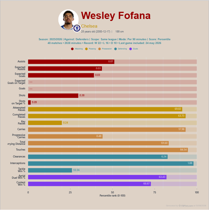
The sensitivity test is simple: raise the eligibility threshold and note which players disappear, then compare totals with per-90 rates. If a headline depends on one low-minute case remaining eligible, the finding is fragile. If the pattern survives several reasonable thresholds, it becomes more suitable for a shortlist—still not a prediction.

Minutes are not a magic quality score either. A large sample can repeatedly reflect the same tactical role, and a small sample can be the only available evidence after injury or transfer. Report what the sample permits, explain what it withholds and make the next data update part of the plan.

An injury return is a good example. The first 300 minutes may reveal that a player is being used in a new position, but they are a weak basis for ranking his stable output against full-season peers. The chart can still enter an internal note if its language matches the evidence: “early usage pattern” is defensible; “new performance level” is not.

The same principle applies to substitutes. Per-90 rates from short appearances can be shaped by open game states and tired opponents. Compare starts with substitute minutes where possible, inspect the match situations and resist multiplying the rate into a hypothetical full season. Normalisation removes unequal exposure from the arithmetic; it does not recreate the missing ninety minutes.

Build the Sensitivity View

Create one coherent FBPlot population, export the baseline, apply a stricter minutes or matches rule and export again. Compare the conclusions, not only the top name. The uncertainty revealed by the second view is part of the analysis.